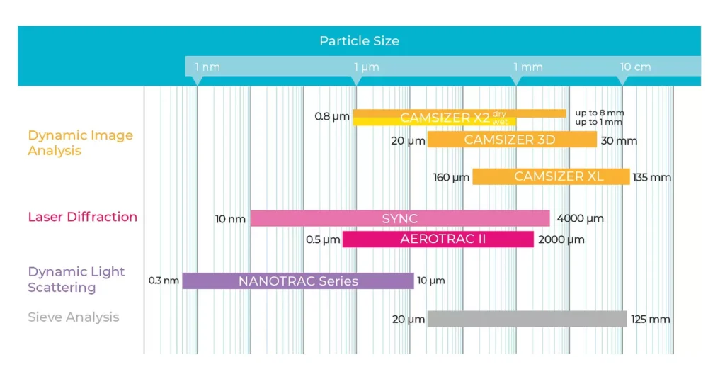
Particle Size Analysis: Comparing DIA, SLS, Sieving & DLS Techniques
4.
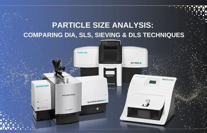
Particle Size Analysis: Comparing DIA, SLS, Sieving & DLS Techniques
-
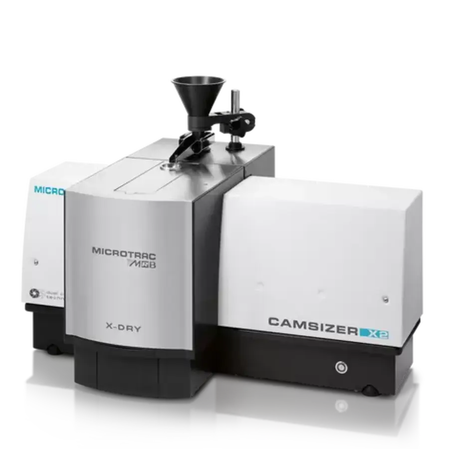
Microtrac CAMSIZER X2 Particle Size and Shape Analyzer
The CAMSIZER X2 is a powerful, extremely versatile particle size and shape analyzer with a wide measuring range.
-
Brand:
Microtrac
-
Brand:
-
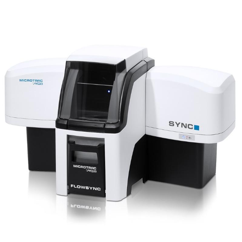
Microtrac SYNC Particle Size and Shape Analyzer
Microtrac SYNC is a particle size and shape analyzer integrating highly accurate tri-laser diffraction analyzer technology with versatile dynamic image...
-
Brand:
Microtrac
-
Brand:

Related Posts